During the last several months, I noticed a lot of discussion about cumulative tropical cyclone activity on a global scale. Record numbers of storms have formed in several tropical basins around the globe in 2015. That's the end of the story, right? Well, there are a number of ways to parse this data. The easiest way to measure tropical cyclone activity is do a simple count. You may then want to measure storms above a certain intensity. A more recent metric (~15 years) is something called Accumulated Cyclone Energy – or ACE for short. The principle behind ACE is to measure the cumulative energy generated by a storm. Since energy is a squared function of the wind speed, ACE accumulates rapidly as a storm intensifies. The formula for ACE at a single moment in time is the wind speed in knots raised to the second power, then divided by 10,000.

If you add all the ACE values during the life history of a storm, a total ACE for that storm is generated. HERE is a running total of ACE, by storm, for the 2015 season from the Weather Underground.
Climatology
Running totals of ACE by season or by basin is very informative, as tropical cyclones are an important mechanism for transporting heat from low latitudes to high latitudes. The more cumulative tropical cyclone activity there is, the more heat transport occurs. It also goes without saying that storm intensity greatly affect the loss of life and property when storms make landfall.
In addition to seasonal charts of ACE, I am interested in the spatial distribution of tropical cyclone activity – specifically, the spatial climatology of ACE. My initial background research into ACE climatology came up empty. No research initiative appeared to address this question directly and no information on ACE climatology exists at any of the national tropical forecast centers. Therefore, I decided to generate ACE climatology maps myself.
Previous Research
After spending a fair amount of effort generating a map set myself, it turns out that such a map does indeed exist. Doh! Oh well. Here is a link to the existing map by (Woodruff et. al, 2013): http://www.nature.com/nature/journal/v504/n7478/fig_tab/nature12855_F1.html . It covers the 1981 to 2010 time period and is in the most prestigious science journal in the world, Nature. I am only providing the link to the map as to not get in trouble for embedding the image directly.
Interestingly, it is merely an aside in an article about coastal flooding potential from tropical cyclones. No discussion is present regarding their methodology and no citations are provided indicating earlier work on the topic. Based on the appearance of the map, it appears that they set up a 2° x 2° grid across the globe and overlaid historical storm tracks over those grid cells. Storms intersecting those grid cells were likely queried for maximum wind speed and an ACE value computed. If this was their methodology, and it probably was, variability of ACE as a function of storm speed would result in a spatial ACE under count. Also, the use of strictly defined bins causes boundary issues depending on the trajectory of storms and the size of the bins. These are not criticisms of the Woodruff et. al study, as developing an ACE climatology was not the focus of their research.
My Study
Imagine you are stranded on a small island in the middle of the Atlantic Ocean (e.g., Dominica). In any given year, how much tropical energy do you expect to encounter? That is what I set out to answer. Consider it a hazardousness-of-place study.
Using the 2° bins from the Woodruff et. al study, any storm entering the 2° space that you reside in will go into a calculation that ultimately leads to a climatological average. Well, what if the 2° bin boundary is 15 miles north of your location and a category 3 hurricane passes 25 miles north of you? The methodology described above would show zero ACE experienced at your location. In reality, much destruction probably occurred and you very well may be clinging to a tree. Therefore, I set out to map ACE by location using a regularly spaced grid of points and employing a search radius from storm positions that allows for overlapping selections.
Figure 1 shows a map with grid points in all six tropical cyclone basins that I generated to develop an ACE climatology. The points are spaced 60 nautical miles apart. A total of 14,498 points were established. Points begin at 5°N/S and extend to 45°N and 40°S. I should note that the point spacing does account for the converging of meridians with increasing latitude. The horizontal distance between points is the same at 40° as it is at 5°.

Methodology
Using a system of trial and error, I settled on a critical search radius of 150 statute miles for analysis from each grid point. A quick way to describe the process is that for each of the 14,498 grid points, I queried the entire IBTrACS tropical climatology database using years with storm information considered highly reliable (for quality and completion). Each time a storm position was within 150 miles of a grid point, the ACE value for that storm observation was assigned to that point. This means every storm position is within the 150-mile domain of at least 4 grid points. The working assumption is that a storm's energy affects an area of at least 150 miles in all directions of a point. Of course tropical cyclone energy decays at a fairly well established rate and that is not accounted for in this study; primarily because individual storm wind field asymmetries and motion vectors are difficult to account for.

Sample Calculation
The map in Figure 2 shows how the calculations were performed using data from the 2008 North Atlantic hurricane season. Two sample points are shown with green triangles and 150-mile buffers are shown around each of the two points.
Within the buffer surrounding the point located at 13.0°N and 86.7°W (central Gulf of Mexico), a total of eight tropical cyclone positions from the 2008 season were captured. Six of those positions are from Hurricane Ike and two of the positions are from Hurricane Gustav. The six points from Hurricane Ike have a combined ACE value of 4.24. The two points from Hurricane Gustav have a combined ACE of 1.90. The total ACE for all storm positions within 150 miles of 13.0°N/86.7°W is 6.14. Even though Gustav was stronger than Ike, its faster forward motion means that fewer storm positions fell within the buffer. This nicely demonstrates that speed impacts the ACE at a location. Slower storms generate more ACE.
The 150-mile buffer surrounding the point located at 28.0°N and 82.0°W had a very different set of storm conditions. Only one storm, Tropical Storm Fay, came within 150 miles of the point. There were 14 storm positions within this buffer with a combined ACE value of 3.535. I should note that this point is over land and probably experienced a lot less ACE than a similarly situated point over water; however, the point was selected only to demonstrate the calculation process.
The eight storm positions in the central Gulf of Mexico had average ACE values of 0.7676. The fourteen storm positions over central Florida had an average ACE value of 0.2525. The speed/duration of a storm is clearly an important piece of information when interpreting the map(s).
Finally, the map shows color shadings for the sum of seasonal ACE at all of the grid point locations. Areas in brown, purple, and white have the highest values while areas in green have the lowest. This is a good time to point out that the sum of ACE for all point is much higher than the seasonal total of adding up the ACE for each storm position since every storm position is captured by at least four grid points. Remember that this is an ACE climatology for 14,498 separate locations – not an ACE climatology per tropical basin.
Results
In consultation with Dr. Phil Klotzbach at Colorado State University, the following years were chosen for analysis in the separate basins:
Northeast and Central Pacific: 1971-present
Northwest Pacific: 1966-present (1977-present due to data constraints)
North Indian Ocean: 1990-present
South Indian Ocean: 1990-present
South Pacific Ocean: 1971-present (1986-present due to data constraints)
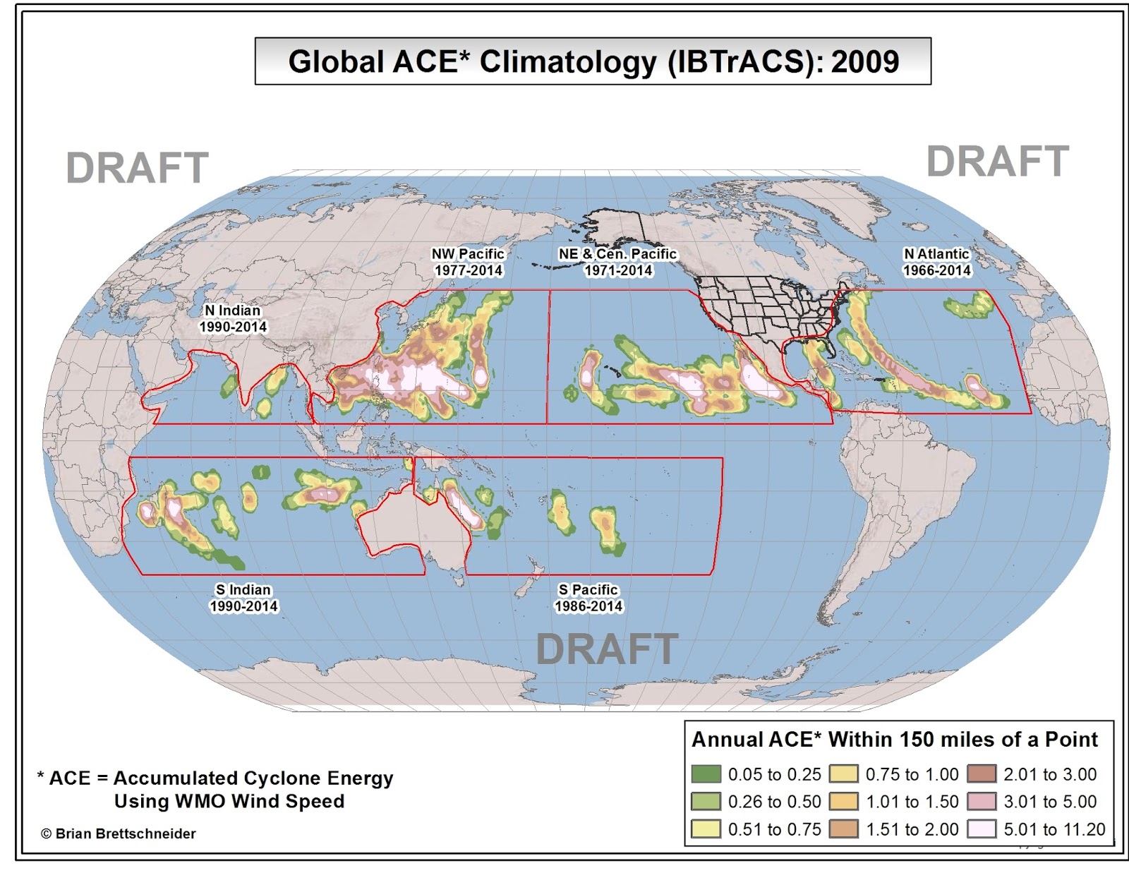
After conducting point-by-point analyses for all grid points in all basins, I came up with the map shown in Figure 3.

As you can see, there is quite a bit of information in the map. The climatology of ACE reflects not only the frequency and speed of storms, but the geographical variability in storm tracks. Also, since tropical cyclones generate their energy from the latent heat stored in oceanic water, ACE is also geographically constrained to regions with relatively warm water (>26.5°C) – at least during the formative stages of their existence.
For example, storms in the Northeast Pacific Basin are geographically clustered to a fairly confined space off the southwest coast of Mexico. Storms in this region are common, achieve high wind speeds, and generally follow the same track. On the other hand, North Atlantic storms are spread out over a much larger area and there are multiple favored storm tracks depending on the season. Northwest Pacific storms are both geographically spread out and quite numerous; therefore; a large area experiences high ACE. In the southern hemisphere, the latitudinal variation in storms is fairly narrow so even with fewer storms, they traverse a similar path; thereby generating high climatological ACE values. A YouTube visualization of year-to-year ACE nicely demonstrates the seasonal variability and also some familiar patterns.
El Niño (MEI)
Variations in seasonal tropical activity have previously been demonstrated to show a high degree of correlation to the presence of an El Niño or a La Niña (Gray, 1984). Shifting pressure and temperature regimes affect water temperatures, wind shear, and a host of other variable that influence the formation and development of tropical systems. During the (near) record 2015 tropical cyclone season in the Northern Hemisphere, activity in the North Atlantic basin was significantly below normal. Other basins responded with hyperactive tropical activity. The MEI in 2015 is at near record levels for the post-1950 era.
Dr. Klotzbach kindly provided two-month values of the Multivariate ENSO Index (MEI) since 1950. The MEI is an El Niño-ish index that describes "the first principal component of six observed fields" (Wolter and Timlin, 1993). Those field are: SLP, zonal and meridional surface wind components, SST, near-surface air temperatures, and total cloudiness.
Each of the years with low, neutral, and high MEI values were processed and grouped together to generate composite maps. An MEI value of +/- 0.75 was used as the threshold for low, neutral, or high. In addition, the MEI was assessed for the main development time for each hemisphere. Therefore, a neutral year in the northern hemisphere may be low, neutral, or high in the southern hemisphere since different months are evaluated for each hemisphere. Figures 5, 6, and 7 show the results of the MEI groupings. Figure 8 shows the difference between the high MEI seasons and the low MEI seasons.

Figure 5. Global ACE climatology for years with neutral MEI values (-0.75<MEI<+0.75).

Figure 6. Global ACE climatology for years with high MEI values (MEI>+0.75).

Figure 7. Global ACE climatology for years with low MEI values (MEI<-0.75).

Figure 8. Difference in ACE between years with high MEI values and low MEI values within 150 miles of a point (MEI High - MEI Low).
There is quite a bit of variability during seasons in different basing according to the MEI index. Low MEI years are more active in the North Atlantic but less active in the North Pacific Basins. The opposite is true in high MEI years. There are also latitudinal shifts. High MEI years tend to have more southerly activity in both hemispheres. There are also many sub-basin differences as well. Too many to mention. I will add to the MEI variability discussion as time permits.
Conclusion
ACE is a tremendously valuable metric for describing tropical cyclone activity. It combines frequency, intensity, and longevity into a single measure. However, there are important spatial components to ACE that are worth examining in closer detail. This (pre-)study is my attempt to further that discussion.
References
Brettschneider, B. 2008: Climatological Hurricane Landfall Probability for the United States. J. Appl. Meteor. Climatol., 47, 704–716. doi: http://dx.doi.org/10.1175/2007JAMC1711.1
Gray, W. M., 1984. Atlantic seasonal hurricane frequency. Part I: El Niño and 30 mb quasi-biennial oscillation influences. Mon. Weath. Rev., 112, 1649-1668.
Knapp, K. R., M. C. Kruk, D. H. Levinson, H. J. Diamond, and C. J.
Neumann (2010), The International Best Track Archive for Climate
Stewardship (IBTrACS): Unifying tropical cyclone best track data,
Bull. Am. Meteorol. Soc., 91, 363–376, doi:10.1175/2009BAMS2755.1
Wolter K, Timlin MS. 1993. Monitoring ENSO in COADS with a seasonally adjusted principal component index. Proceedings of the 17th Climate Diagnostics Workshop, Norman, OK,NOAA/NMC/CAC, NSSL, Oklahoma Climate Survey, CIMMS and the School of Meteorology, University of Oklahoma: Norman, OK;52–57.
Woodruff, J. D., J. L. Irish, and S. J. Camargo. (2013), Coastal flooding by tropical cyclones and sea-level rise. Nature 504, 44–52 doi:10.1038/nature12855
Additional Maps
The following forty-nine (49) maps show the ACE for each calendar year. You can click on each image to see an enlarged version of the map.